Genomic Selection for Adjacent Genetic Markers of Yorkshire Pigs Using Regularized Regression Approaches

Minsu Park; Tae-Hun Kim; Eun-Seok Cho; Heebal Kim; Hee-Seok Oh

doi:10.5713/ajas.2014.14236

Abstract

This study considers a problem of genomic selection (GS) for adjacent genetic markers of Yorkshire pigs which are typically correlated. The GS has been widely used to efficiently estimate target variables such as molecular breeding values using markers across the entire genome. Recently, GS has been applied to animals as well as plants, especially to pigs. For efficient selection of variables with specific traits in pig breeding, it is required that any such variable selection retains some properties: i) it produces a simple model by identifying insignificant variables; ii) it improves the accuracy of the prediction of future data; and iii) it is feasible to handle high-dimensional data in which the number of variables is larger than the number of observations. In this paper, we applied several variable selection methods including least absolute shrinkage and selection operator (LASSO), fused LASSO and elastic net to data with 47K single nucleotide polymorphisms and litter size for 519 observed sows. Based on experiments, we observed that the fused LASSO outperforms other approaches.

Keywords: Genomic Selection; Pig; Litter Size; Single Nucleotide Polymorphism; Regularized Regression

INTRODUCTION

Genomic selection (GS) has been substantially developed in the last few years (Usai et al., 2009; Ogutu et al., 2012), which estimates the total genetic value for animals utilizing the genomic information of a dense marker map covering all the chromosomes (Meuwissen et al., 2001). In practice, GS has been applied in an attempt to increase the accuracy of breeding values in various fields such as crop and livestock breeding (Ibañez-Escriche and Gonzalez-Recio, 2011; Ogutu et al., 2012; Würschum et al., 2013). For pig breeding, the different implementations of GS have been conducted to increase in accuracy of the breeding values (Simianer, 2009; Cleveland et al., 2010; Lillehammer et al., 2013). As interest in GS increased, the computational cost and the prediction accuracy of GS become important issues especially when the data are high-dimensional, i.e., the number of variables is larger than the number of observations.

Previously genome-wide association studies that utilize individual genes or a few quantitative trait loci (QTL) were popular (Meuwissen et al., 2001; Dekkers, 2002). However, it has a limitation in that it cannot reflect the effects of the neighborhood variables. In fact, the single nucleotide polymorphisms (SNPs) are ordered by physical locations on the chromosomes, therefore, adjacent SNPs are correlated with similar associations (Liu, 2011).

The main objective of this study is to provide significant SNPs that affect the average litter size of Yorkshire pigs using regularized regression approaches and to predict the litter values with selected SNPs in the final model. To accommodate the above property of SNPs properly, we consider some regularized regression approaches: least absolute shrinkage and selection operator (LASSO) (Tibshirani, 1996), fused LASSO (Tibshirani et al., 2005), and elastic net (Zou and Hastie, 2005). It is well known that these methods identify significant variables efficiently, improve the accuracy of the prediction and handle high-dimensional data simultaneously.

In fact, Ogutu et al. (2012) performed gnomic selection using some regularized regression methods. However, there are some key features that distinguish this study from Ogutu et al. (2012). First, in this study, we have analyzed ultrahigh-dimensional data that contain 519 sows with 47,112 SNPs, while Ogutu et al. (2012) considered a dataset that has 3,000 observations with 9,990 SNPs. It is well known that the performance of regularized regressions varies over the degree of dimensionality. Thus, this study can be considered as an extension of high-dimensional case of Ogutu et al. (2012). Second, an important issue of regularized regressions is their implementation when the data are high-dimensional, because it heavily involves solving optimization. To handle such ultrahigh-dimensional data, we have used three regularized regression methods with efficient algorithms introduced by Liu et al. (2010); and hence, many researchers can easily implement the methods for GS with various high-dimensional data. Finally, we have focused on the fussed LASSO. It is designed for a problem with features that can be ordered in some meaningful ways as well as a dataset where the number of features is much greater than the sample size. The abovementioned issues can be considered as main contributions of this study.

MATERIALS AND METHODS

The Rural Development Administration (RDA) provided the Illumina Porcine 60K SNP Beadchip on 703 sows and their litter size. Since this study is focused on the litter values of pigs, multiparous sows were used in the analyses. In this section, we explain the details of data in the analysis and the methods used for analysis.

Data

The original genotype data consisted of 60K SNP markers of 703 sows. Samples were excluded if they had a missing genotype rate (>0.05) per sample, and genotype data were also removed if they had low minor allele frequency (<0.01) or significant deviation from the Hardy-Weinberg equilibrium (p<0.0001) as determined by the Plink whole genome analysis toolset (Purcell et al., 2007). A quality control was performed when each SNP was recoded as having a value of 0, 1, or 2 for analysis.

There are several phenotype traits that genetically superior animals hold such as litter size by parity, gestation length, and number born alive. We considered the average litter size for sows as the response variable and the Illumina Porcine 60K SNPs as the independent variables. Although litter size is a trait with low heritability in pigs, it seems that, in our dataset, the litter size is the only response variable that could be used in regression models without imputation of feature variables (SNPs) and removing lots of pigs. The choice of response variable is not main issue of this study. As mentioned earlier, the main purpose of the paper is to compare the performance of three regularized regressions and to extract the influence SNPs for a particular trait when the data are ultrahigh-dimensional; and hence, it is feasible to use other traits that represent the productivity of pigs when such data are available.

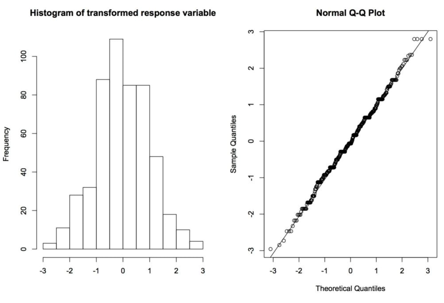
Litter size by parity in pigs is defined as the number of piglets born at a time and the parity of observed litter size in this data set ranges from 1 to 12. The observed objects per parity among a total of 4,163 pigs are described in Figure 1. The more the parity increases, the fewer objects there are (Figure 1). As shown in Figure 2, litter size per parity is almost identical as proved using the Tukey’s honestly significant difference test. Therefore, in this analysis, we consider the average litter size for each sample matched with the objects of SNP marker information. The average values of litter size that can be addressed via the response variable must satisfy the Gaussianity assumption. To comply with this assumption, we used the Box-Cox transformation which chooses an optimal transformation to rectify deviations from the assumption. Figure 3 shows the empirical distribution of the transformed variable that satisfies the Gaussianity assumption. The Shapiro-Wilk normality test (Royston, 1982) gave a p-value of 0.3 with Shapiro-Wilk statistics of 0.9856. It implies that we cannot reject the Gaussianity assumption at the 0.05 significance level.

After phenotype and genotype realignment, the data set consists of 47,112 SNPs out of a total of 61,177 SNPs markers and 519 sows qualified for GS.

Figure 1

Observed sows per parity. The range of parity has from 1 to 12 and initial distinct observations having litter size values are 4,163 Yorkshire sows.

Figure 2

Boxplot of litter size per parity. Boxplot depicts the distribution of the sows per parity through their quartiles. The black line in box represents the second quantile (median) of litter size and the upper and lower boundary of box means third quantile and first quantile, respectively.

Figure 3

Identification of the Gaussian assumption. The empirical distribution of transformed average litter size by the Box-Cox transformation (left) and the normal Q-Q plot comparing randomly generated by independent normal data to the standard normal population (right).

Methods

The linear model for the genetic effects at adjacent SNPs is

y=Xβ+ɛ

where y is an n×1 vector of observed average litter size, X is an n×p matrix of genotypes, and β is a p×1 vector of the regression coefficients of the SNP markers. Here, ɛ is an n×1 vector of the i.i.d. random errors with ɛ~N(0,Iσɛ2), where σɛ2 denotes a constant variance.

LASSO (Tibshirani, 1996)

LASSO has been widely used for variable selection. It is used to find regression coefficients β that minimizes the usual sum of squared errors with a constraint on the sum of the absolute values of the coefficients as follows

β^=arg minβ‖y-Xβ‖2+Pλ(β)

where the penalty function is P_λ(β) = λ||β||_l_₁ with a regularization parameter λ≥0. Although LASSO is efficient and has a fast algorithm, it tends to arbitrarily select only one variable from the group when adjacent SNPs have pairwise high correlations, which may not be suitable for our analysis.

Fused LASSO (Tibshirani et al., 2005)

Fused LASSO is designed for a proper group selection that may be suitable for this study. The fused LASSO is defined as

As shown in the above criterion, the fused LASSO requires a natural ordering of the independent variables for integrating correlated variables well. The physical ordering of SNP markers across a chromosome is simply satisfied.

Elastic net (Zou and Hastie, 2005)

Elastic net is a regularized regression method that can be considered as an extension of LASSO. The penalty of elastic net consists of l₁ and l₂ parts, which means that it is a mixture of LASSO and ridge regression penalties. The quadratic penalty part captures the group of highly correlated variables, and hence, it overcomes a limitation of LASSO. The elastic net estimator can be expressed as

β^(EN)=arg minβ‖y-Xβ‖2+λ1‖β‖1+λ2‖β‖22.

Letting α = λ₂/(λ₁+λ₂), the estimator is equivalent to the following optimization problem:

β^(EN)=arg minβ‖y-Xβ‖2,

subject to (1-α)‖β‖1+α‖β‖22≤t for some t.

Comparing methods

Since the optimizations for LASSO, fused LASSO, and elastic net involve a non-linear procedure, finding the solutions is not trivial (Tibshirani and Taylor, 2011). To improve the speed and the accuracy of the solution paths, we used the efficient algorithm by Liu et al. (2010) with the accelerated gradient method of Nesterov (2007) and a two-deep 10-fold cross-validation (CV) in MATLAB as follows:

Partition the data into the first-deep training and validation sets; then partition the first-deep training set into the second-deep training and test set (two-deep CV).
At the second-deep, construct the model using the sub-training set and calculate CV; then choose the optimal tuning parameter that minimizes CV.
At the first-deep, fit the model and estimate the coefficients in the first-deep training set with the estimated regularization parameter from the second-deep set.

To evaluate the regularized regressions described in Section 2, we calculated the prediction error (PE), which is defined as

PE=‖yval-Xvalβ^tra‖2nval

where the subindex val implies the validation set, β̂_tra is a vector of the coefficients obtained from the first-deep training set and X_valβ̂_tra denotes a vector of the predicted values on the validation set. As a standard criterion for the performance, we consider mean fitting prediction error (MFPE) which replaces X_valβ̂_tra in the definition of PE with ȳ_tra.

RESULT AND DISCUSSION

To compare the performance of the three methods, PE and the Pearson correlation between the true litter values and the predicted values were used as measures of the accuracy. The number of non-zero coefficients was also used as an indicator of efficiency. If the structure of the training set is totally different from the arrangement of the validation set because of the limitation of data, then the evaluation of the method might not be reliable. To clarify the comparison for the results of methods, we extracted new samples from the original data using the bootstrap technique with a 35% resampling rate.

The overall results of each method with partitioned bootstrap samples are presented in Table 1 to 3. Table 1 describes PEs by LASSO, fused LASSO, and elastic net, and MFPE for each fold. The average PEs obtained by LASSO, fused LASSO, and elastic net were 0.8675, 0.8476, and 0.8628, respectively. As listed, the fused LASSO outperformed other methods when the explanatory variables were correlated. From Table 2, the fused LASSO provided the highest accuracy over all folds. Table 3 lists the number of non-zero coefficients selected by LASSO, fused LASSO, and elastic net. Overall, the number of non-zero coefficients by the fused LASSO was slightly high, compared to LASSO and elastic net. In the case of fold 4, for example, the consecutively selected variables by the fused LASSO were DRGA0005762, DRGA0005763, DRGA0005767, and DRGA0005770, while the LASSO selected only DRGA0005770. According to the results of the above comparison study, the fused LASSO performed well. Ogutu et al. (2012) analyzed a dataset with 9,900 SNP markers on 3,000 progenies of 20 sires and 200 dams by using various GS methods such as ridge regression, ridge regression best linear unbiased prediction (BLUP), LASSO, adaptive LASSO, elastic net, and adaptive elastic net. In their analysis, elastic net and LASSO worked well for GS, compared to others.

Table 1

PE1 and average PE by regularized regressions and MFPE2

Fold	MFPE	Regularized regression

		LASSO	Fused LASSO	Elastic net
1	1.0061	0.9673	0.9514	0.9610
2	0.9796	0.8052	0.7777	0.7794
3	0.8429	0.7227	0.7049	0.7210
4	0.9595	0.8370	0.8172	0.8306
5	1.0420	0.8282	0.8061	0.8257
6	1.0147	0.9110	0.8885	0.9236
7	1.0813	0.9950	0.9809	0.9918
8	1.0241	0.8880	0.8635	0.8851
9	1.0163	0.8972	0.8784	0.8931
10	0.9568	0.8235	0.8074	0.8169
Ave PE	0.9923	0.8675	0.8476	0.8628

PE, prediction error; MFPE, mean fitting prediction error; LASSO, least absolute shrinkage and selection operator; Ave PE, average prediction error for fold.

¹ The root mean squared error with respect to fitted coefficients from the first-deep training set.

² The root mean squared error with respect to fitted mean of litter size from the first-deep training set.

Table 2

Accuracy (Pearson correlation1) and average correlation by regularized regression methods

Fold	Regularized regression

	LASSO	Fused LASSO	Elastic net
1	0.3627	0.4150	0.3972
2	0.6802	0.6978	0.6966
3	0.6136	0.6410	0.6239
4	0.5600	0.5848	0.5694
5	0.7295	0.7510	0.7338
6	0.5973	0.6265	0.6011
7	0.4849	0.5126	0.4925
8	0.5931	0.6070	0.5962
9	0.5200	0.5422	0.5291
10	0.5708	0.5891	0.5777
Ave corr1	0.5712	0.5967	0.5818

LASSO, least absolute shrinkage and selection operator; Ave corr, average Pearson correlation for fold.

¹ Pearson correlation coefficient is obtained by the true litter size vectors in validation set and predicted values which coefficients in the model are derived from training set at each fold.

Table 3

Number of non-zero estimated coefficients derived from training set by regularized regression methods (total SNPs: 47,112)

Fold	Regularized regression

	LASSO	Fused LASSO	Elastic net
1	445	884	903
2	850	847	678
3	499	759	863
4	510	514	368
5	535	851	601
6	553	821	869
7	949	1,339	1,035
8	1,056	963	1,139
9	917	850	1,004
10	899	1369	620
Ave numb¹	721.3	953.3	808

LASSO, least absolute shrinkage and selection operator; Ave numb, average number.

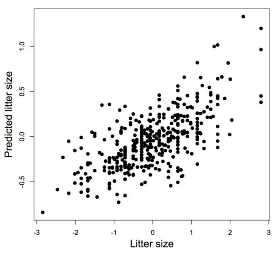
To construct the final model, we used the whole data set, and calculated PEs and correlation values between the given target variable and the predicted value to indicate accuracy. In the results of the final model obtained by the fused LASSO, the number of significant non-zero coefficients among 47,112 SNPs was 1,499 SNPs. Table 4 lists the names of the 10 selected significant SNPs with large estimated coefficients (in absolute value) of the SNP effects. Onteru et al. (2012) provided some important genes for reproductive traits in the QTL regions, where they employed the Bayes C model introduced by Kizilkaya et al. (2010). Figure 4 shows the scatter plot between the predicted values ŷ and the original values y. Note that the sample correlation coefficient between litter size and predicted litter size by the final model was 0.7041. It seems that the fused LASSO is suitable for selecting adjacent SNPs as well as for predicting the values.

In summary, we have considered three regularized regressions for GS with 47,112 SNPs of 519 sows. We compared three methods using PEs and correlation coefficient values, and obtained the final model to predict the litter size of pigs. From the data analysis, we observed that the fused LASSO seems to be a good choice for GS.

Figure 4

Scatter plot of true average litter size and predicted litter size obtained by the fused LASSO in the final model. The sample correlation coefficient is 0.7041. LASSO, least absolute shrinkage and selection operator.

Table 4

The 10 SNPs with the highest coefficients (in absolute value) selected by the fused LASSO1

Name of SNP	Coef2
M1GA0023299	0.0099
MARC0015851	0.0094
H3GA0002658	0.0084
ASGA0001125	0.0074
ALGA0106999	0.0069
MARC0016306	0.0068
ASGA0080059	0.0064
ASGA0054467	−0.0063
MARC0027886	−0.0064
MARC0023564	−0.0064

SNP, single nucleotide polymorphism; LASSO, least absolute shrinkage and selection operator.

¹ The significant SNPs in the final model are obtained from the whole data set using the fused LASSO.

² Estimated coefficient by the fused LASSO.

Finally, the regression methods for estimating the random effect in a mixed model have recently developed (Onteru et al., 2012; Resende et al., 2012). As a future study, it is worth confirming the effects of a random effect model compared to existing GS methods.

REFERENCES

Cleveland M, Forni S, Garrick DJ, Deeb N. 2010. Prediction of genomic breeding values in a commercial pig population. In : Proc 9th World Congr. Genet. Appl. Livest. Prod; Leipzig, Germany.
Dekkers J. 2002. The use of molecular genetics in the improvement of agricultural populations. Nat Rev Genet 3:22–32.
crossref pmid
Ibañez-Escriche N, Gonzalez-Recio O. 2011. Review. Promises, pitfalls and challenges of genomic selection in breeding programs. Span J Agric Res 9:404–413.
crossref
Kizilkaya K, Fernando RL, Garrick DJ. 2010. Genomic prediction of simulated multibreed and purebred performance using observed fifty thousand single nucleotide polymorphism genotypes. J Anim Sci 88:544–551.
Lillehammer M, Meuwissen THE, Sonesson AK. 2013. Genomic selection for two traits in a maternal pig breeding scheme. J Anim Sci 91:3079–3087.
Liu J. 2011. Penalized Methods in Genome-wide Association Studies. PhD Thesis. University of Iowa; Iowa City, IA, USA:
Liu J, Yuan L, Ye J. 2010. An efficient algorithm for a class of fused LASSO problems. Advances in Neural Information Processing Systems (NIPS). Curran Associates, Inc; Vancouver, BC, Canada:
Meuwissen THE, Hayes BJ, Goddard ME. 2001. Prediction of total genetic value using genome-wide dense marker maps. Genetics 157:1819–1829.
crossref pmid pmc pdf
Nesterov Y. 2007. Gradient methods for minimizing composite objective function. CORE Discussion Paper 76.
Ogutu JO, Schulz-Streeck T, Piepho HP. 2012. Genomic selection using regularized linear regression models: Ridge regression, lasso, elastic net and their extensions. BMC Proc 6:Suppl 2S10
crossref pmid pmc
Onteru SK, Fan B, Du ZQ, Garrick DJ, Stalder KJ, Rothschild MF. 2012. A whole-genome association study for pig reproductive traits. Anim Genet 43:18–26.
Purcell S, Neale B, Todd-Brown K, Thomas L, Ferreira M. 2007. PLINK: A tool set for whole-genome association and population-based linkage analyses. Am J Hum Genet 81:559–575.
Resende MFR, Munoz P, Resende MDV, Garrick DJ, Fernando RL, Davis JM, Jokela EJ, Martin TA, Peter GF, Kirst M. 2012. Accuracy of genomic selection methods in a standard data set of loblolly pine (Pinus taeda L.). Genetics 190:1503–1510.
Royston JP. 1982. An extension of Shapiro and Wilk’s W test for normality to large samples. J Appl Statist 31:115–124.
Simianer H. 2009. The potential of genomic selection to improve litter size in pig breeding programs. In : Proc 60th Annual Meeting of the European Association of Animal Production; Barcelona, Spain.
Tibshirani R. 1996. Regression shrinkage and selection via the LASSO. J R Statist Soc Ser B 58:267–288.
Tibshirani R, Saunders M, Zhu J, Knight K. 2005. Sparsity and smoothness via the fused LASSO. J R Statist Soc Ser B 67:91–108.
Tibshirani R, Taylor J. 2011. The solution path of the generalized LASSO. Ann Stat 39:1335–1371.
Usai MG, Goddard ME, Hayes BJ. 2009. LASSO with cross-validation for genomic selection. Genet. Res (Cambridge) 91:427–436.
Würschum T, Reif JC, Kraft T, Janssen G, Zhao Y. 2013. Genomic selection in sugar beet breeding populations. BMC Genet 14:85
Zou H, Hastie T. 2005. Regularization and variable selection via the elastic net. J R Stat Soc Ser B 67:301–320.
Editorial Office
Asian-Australasian Association of Animal Production Societies(AAAP)
Room 708 Sammo Sporex, 23, Sillim-ro 59-gil, Gwanak-gu, Seoul 08776, Korea
TEL : +82-2-888-6558    FAX : +82-2-888-6559
E-mail : editor@animbiosci.org
Copyright © 2024 by Asian-Australasian Association of Animal Production Societies.
Developed in M2PI