Predicting the rate of inbreeding in populations undergoing four-path selection on genomically enhanced breeding values

Prediction of expected long-term genetic contributions

Our prediction method is based on the concept of long-term genetic contributions. The long-term genetic contribution of individual i (r_i) in generation t₁ is defined as the proportion of genes from individual i that are present in individuals in generation t₂ deriving by descent from individual i, where (t₂–t₁) →∞ [5]. That is, after several generations, the genetic contributions of ancestors stabilize and become equal for all descendants, i.e., the ultimate proportional contribution of an ancestor to its descendants is reached.

Selection is performed in four categories of selection path (SS, SD, DS, and DD). Rates of inbreeding can be expressed in terms of the expected contributions of these categories [6, 9–11]:

where 1′ = (1 1 1 1), N is a 4×4 diagonal matrix containing the number of selected parents for element (i, i) as N_i,i, N_1,1 is the number of sires in SS and is referred to as N_SS, N_2,2 is the number of sires in SD and is referred to as N_SD, N_3,3 is the number of dams in DS and is referred to as N_DS, and N_4,4 is the number of dams in DD and is referred to as N_DD. In addition, u2=(ui,SS2 ui,SD2 ui,DS2 ui,DD2), where u_i,SS is the expected lifetime long-term genetic contribution of individual i in category SS conditional on its selective advantage (which in mass selection is the genomically enhanced breeding value [GEBV]), and u_i,SD, u_i,DS, and u_i,DD are the expected lifetime long-term genetic contributions of individual i in categories SD, DS, and DD, respectively. Furthermore, δ = (δ_SS δ_SD δ_DS δ_DD), where δ_SS is the correction factor for deviations of the variance of family size from independent Poisson variances in the selected offspring from sires in SS; δ_SD, δ_DS, and δ_DD are corrections for deviations of the variance of the family size from independent Poisson variances in the selected offspring from parents in SD, DS, and DD, respectively.

The selective advantage of the ith sire in SS (S_i,SS) and in SD (S_i,SD) in the linear model is:

where A_i,SS is the breeding value of sire i in SS or SD, Ā_{i,DS and DD} is the average breeding value of dams mated to the ith sire in SS and SD, respectively; the dams mated to the ith sire in SS belong to the DS category, and the dams mated to the ith sire in SD belong to the DD category; and Ā_i,SS, Ā_i,SD, Ā_i,DS, and Ā_i,DD, are the average breeding values of the individuals in the SS, SD, DS, and DD categories.

The selective advantage of the ith dam in DS (S_i,DS) and in DD (S_i,DD) in the linear model is:

where A_{i,DS and DD} is the breeding value of dam i in DS and DD, respectively; A_{i,SS and SD} is the breeding value of a sire mated to the ith dam in DS and DD, respectively; the sires mated to the ith dam in DS belong to the SS category; and the sires mated to the ith dam in DD belong to the SD category.

Expected contributions (u_{i,SS,SD,DS,or DD}) are predicted by linear regression on the selective advantage. That is,

where α_x is the expected contribution of an average parent in x, and β_x is the regression coefficient of the contribution of i on its selective advantage (S_i,x). In addition, α_x can be obtained according to Woolliams et al [9]:

where G is a 4×4 matrix representing the parental origin of genes of selected offspring in the order of SS, SD, DS, and DD category, i.e., representing rows offspring and columns parental categories. That is,

However,

where α′N is the left eigenvector of G with eigenvalue 1; the left eigenvector is obtained according to Bijma and Woolliams [11] and is equal to (0.25 0.25 0.25 0.25).

Solutions for β_x are obtained according to Woolliams et al [9]:

note that the right hand side of (1) is unaffected by the number of parents, so that β_x is inversely proportional to the number of parents (that is, 1NSS,1NSD,1NDS and 1NDD), where, I₄ is a 4×4 identity matrix, Π is a 4×4 matrix of regression coefficients with π_xy being the regression coefficient of S_i,x of a selected offspring i of category x (SS, SD, DS, DD) on s_j,y of its parent j of category y (SS, SD, DS, DD). For example, π_SD,SS is the regression coefficient of S_i,SD of a selected offspring i of SD on S_j,SS of its parent j of SS. Given that SS is the sires to breed sons category, we have non-zero elements, π_SS,SS and π_SD,SS, in Π as elements (1,1) and (2,1), respectively. In the same way, since SD is the sires to breed daughters category, we have non-zero elements, π_DS,SD and π_DD,SD, in Π as elements (3,2) and (4,2), respectively. Because DS is the dams to breed sons category, we have non-zero elements, π_SS,DS and π_SD,DS, in Π as elements (1,3) and (2,3), respectively. And given that DD is the dams to breed daughters category, we have non-zero elements, π_DS,DD and π_DD,DD, in Π as elements (3,4) and (4,4), respectively.

In addition, Λ is a 4×4 matrix of regression coefficients, with λ_xy being the regression coefficient of the number of selected offspring of category x on S_j,y of its parent j of category y. In the same way as Π, we have non-zero elements, λ_SS,SS and λ_SD,SS, λ_DS,SD and λ_DD,SD, λ_SS,DS and λ_SD,DS, and λ_DS,DD and λ_DD,DD in Λ as elements (1,1) and (2,1), (3,2) and (4,2), (1,3) and (2,3), and (3,4) and (4,4), respectively. Consequently,

representing rows as offspring and columns as parental categories.

In our current study, elements in matrices Π and λ were calculated from Woolliams et al [9] and Bijma and Woolliams [11], as outlined in Appendices A and B.

The sires in the SS category are included among the sires in SD category. That is, the sires in the SS category are selected not only to breed sons but as sires in the SD category to breed daughters. Similarly the dams in the DS category are included among the dams in the DD category. The dams in the DS category are selected not only to breed sons but as dams in the DD category to breed daughters. Therefore, after applying the procedure of Bijma and Woolliams [6], the number of sires in SD is larger than that of sires in SS, and the number of dams in DD is larger than that of dams in DS. Therefore, E (ΔF)=12(1′N0U01), where

E denotes the expectation with respect to the selective advantage,

and E(Ā_DS – Ā_DD) = (i_DS – i_DD)σ_A,f,

note that variance of selective advantage ( σSS2,σSD2,σDS2, and σDD2) is not affected greatly by the number of parents (N_SS, N_SD, N_DS, and N_DD), since the term of (1-1Nx) is adjustment for finite population size, where σA,m2 and σA,f2 are the equilibrium genetic variance in the male and female populations, respectively; rA^,m2 and rA^f2 are the equilibrium reliability of GEBV in the male and female populations, respectively; and k_SS, k_SD, k_DS, and k_DD are variance reduction coefficients for offspring selection in SS, SD, DS, and DD, respectively. Note that covariances of mates between SS and SD and between DS and DD are zero, because of random mating. General predictions of expected genetic contributions was developed using equilibrium genetic variances instead of second generation genetic variances [9]. Therefore, variances thereafter refer to those in equilibrium.

The accounting percentage derived from SS, SD, DS, and DD for the rate of inbreeding (ΔF) is obtained,

When the effect of selection on inbreeding is ignored, i.e., β = 0, E (ΔF)=12(1′N0U01)=132(1NSS+3NSD+1NDS+3NDD).

This result is in agreement with the formula from Gowe et al [8], which likewise neglects the effects of selection on ΔF.

Correction of E (ΔF) from Poisson variances

The correction for deviations of the variance of the family size from independent Poisson variances in the selected offspring from SS, SD, DS, and DD parents, i.e., δ_SS, δ_SD, δ_DS, and δ_DD, can be approximated by Woolliams and Bijma [10].

According to Woolliams and Bijma [10],

Where

ΔV_SS, ΔV_SD, ΔV_DS, and ΔV_DD, are 4×4 matrices which are variances of selected family size deviated from Poisson variance by applying binomial distribution to the family size from the parents of SS, SD, DS, and DD, respectively, and s_x is the selective advantage of parents in category x (SS, SD, DS, DD). Elements of ΔV_{SS,SD,DS,or DD} are shown in Appendix C.

Example applications of the formula

To demonstrate the application of our formula, we assumed only two quantitative traits: trait 1 was assumed to be moderately heritable, with h² = 0.3, whereas trait 2 was assumed to have low heritability, with h² = 0.1. These traits are selected as single traits expressed as GEBV. Furthermore, we assumed an aggregate genotype as a linear combination of genetic values, each weighted by the relative economic weights, which was expressed as a₁g₁ + a₂g₂, where g₁ is the true genetic value for trait i, a_i is the relative economic weight for trait i, and the genetic correlation between traits 1 and 2 was assumed as 0.4. Index selection was performed to select a₁g₁ + a₂g₂, that is, breeding goal (H), under the assumption that the relative economic weight between traits 1 and 2 is 1:1. Breeding value (A) was defined as described earlier in the Methods; for example, the breeding value of sire i in SS was defined as A_i,SS. Similarly, the breeding goal value (H) of sire i in SS can be expressed as H_i,SS; note that the formula that we developed in Methods can be applied not only to breeding value (A) but also to breeding goal value (H).

In our example, we assumed the reliabilities of the GEBVs for traits 1 and 2 to be 0.5721 and 0.4836, respectively [3]. Index selection (I) was performed as I = a₁ GEBV₁ + a₁ GEBV₂, because GEBVs are assumed to be derived from multiple-trait BLUP (MT BLUP) genetic evaluation methods in the current study (as done for single-step genomic BLUP [13]). We calculated equilibrium genetic variances and reliabilities based on Togashi et al [3]. The initial (generation 0) and equilibrium genetic variances and reliabilities for single-trait selection (h² = 0.3 or h² = 0.1) and index selection are shown in Table 1. Rates of inbreeding were calculated based on equilibrium genetic variances and reliabilities, because regression coefficients of the number or breeding value of selected offspring on the breeding value of the parent are equal for the parental and offspring generations under equilibrium genetic variances and reliabilities.

Table 1

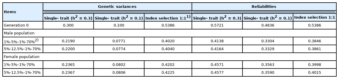
Genetic variances and reliabilities of genomically enhanced breeding values in generation 0 and at the asymptote

We considered two scenarios for the selection percentages for SS, SD, DS, and DD—5%-12.5%–1%-70% and 1%-5%–1%-70%—and three scenarios for the numbers of selected parents of SS, SD, DS, and DD—namely 20-50–100-7,000, 40-100–200-14,000, and 60-150–300-21,000. Therefore, we considered six scenarios (two scenarios of selection percentage and three scenarios of the number of parents in SS, SD, DS, DD) in total. Note that the two scenarios for selection percentage for SS, SD, DS, and DD differ only in the selection percentage along the SS and SD selection paths, because under actual breeding conditions, selection intensity can be adjusted more easily in male selection paths (SS and SD) than in female selection paths (DS and DD). The numbers of male and female offspring from a dam of DS, i.e., fmds and ffds, were set at 4. The number of female offspring from a dam of DD, i.e., ffdd, was set at 1.4. These numbers are derived from the years of usage of a dam and the reproduction method (ovum collection, in vitro fertilization, or embryo transfer). When DS and DD parents are used with constant selection intensity and in equal numbers over several years, they belong to a single or exclusive category. The numbers are used to compute the deviation of the variance of the family size from Poisson variance.

Rates of inbreeding

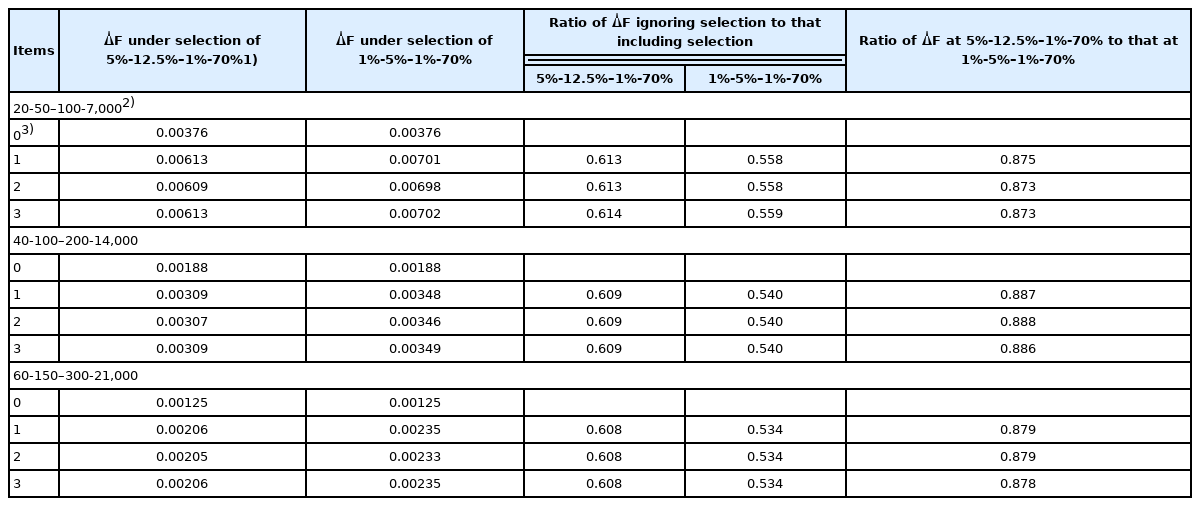
The rates of inbreeding without correction for deviation from Poisson variances (that is, the rates of inbreeding with Poisson family size) are shown in Table 2. Because the rates from Gowe et al [8] do not account for selection, ΔF is the same between two selection percentages in SS, SD, DS, and DD, i.e., 1%-5%–1%-70% and 5%-12.5%–1%-70%. In contrast, ΔF derived from the method developed in the current study increased with the increase in selection intensity. When we applied our formula, ΔF was lower when selection was ignored than when it was included, suggesting that ΔF was underestimated when selection was ignored. The ratio of ΔF when selection was ignored to that when it was included was about 0.61 under the selection percentages of 5%-12.5%–1%-70% for the SS, SD, DS, and DD selection paths, whereas the ΔF ratio was 0.53 to 0.56 under the selection percentage condition of 1%-5%–1%-70%. That is, calculation according to Gowe et al [8] underestimated ΔF by approximately 40% and 45% under selection percentages of 5%-12.5%–1%-70% and 1%-5%–1%-70% for the SS, SD, DS, and DD selection paths, respectively. In contrast, the rates of inbreeding under selection estimated by using our formula were 63% to 87% greater than those calculated according to the current working formula, which does not consider selection [8]. The ratio of ΔF for 5%-12.5%–1%-70% to that for 1%-5%–1%-70% was 0.88 to 0.89, resulting in an approximately 12% decrease in ΔF due to increasing the selection percentage or decreasing the selection intensity for SS and SD for all three scenarios compared in the numbers of parents in SS, SD, DS, and DD (20-50–100-7,000, 40-100–200-14,000, and 60-150–300-21,000). In contrast, the decrease in ΔF due to the increase in the number of parents was proportional to the numbers. The ΔF under the number of parents in SS, SD, DS, and DD (40-100–200-14,000 and 60-150–300-21,000) was approximately half and one third of the ΔF under the number of parents (20-50–100-7,000), respectively, for all two scenarios compared in the selection percentage of parents in SS, SD, DS, and DD (5%-12.5%–1%-70% and 1%-5%–1%-70%). Consequently, the decrease in the rate of inbreeding likely would be greater with an increase in the number of parents than with a decrease in selection intensity; however, we need to perform more trials at different selection intensities to confirm this association.

Table 2

Rate of inbreeding

In general, both genetic gain and ΔF increase with an in crease in selection intensity. However, because the number of parents has a greater effect on inbreeding than does selection intensity, increasing the number of parents is one option for offsetting the increase in ΔF due to an increase in selection intensity.

The rate of inbreeding was slightly lower in single-trait se lection with a low heritable trait (h² = 0.1) than the other selection methods (i.e., single-trait selection with a trait (h² = 0.3) and index selection [Table 2]). However, the difference was not so remarkable. Consequently, we consider the major factors in the rate of inbreeding to be the number of parents and the selection intensity in each of the four selection paths.

Values for effective population size expressed as NE=12ΔF are shown in Table 3. Using a method that ignores selection [8] overestimated the effective population size due to ΔF compared with that computed by using our formula, which accounts for selection. The overestimation was greater when the selection percentage in SS, SD, DS, and DD was 1%-5%–1%-70% than when it was 5%-12.5%–1%-70%. The ratio of NE for the 5%-12.5%–1%-70% condition to that for 1%-5%–1%-70% became greater as the numbers of parents in SS, SD, DS, and DD increased from 20-50–100-7,000 to 40-100–200-14,000 and then to 60-150–300-21,000. This pattern is consistent with the suggestion that increasing the number of parents is one option for offsetting an increase in ΔF due to an increase in selection intensity (Table 2). That is, decreasing ΔF is equivalent to increasing the effective population size.

Table 3

Effective population size (N_E)

The expectation of the square of long-term contribution of an individual (that is, E (ui,SS2), E (ui,SD2), E (ui,DS2), and E (ui,DD2)) in SS, SD, DS, and DD are shown in Table 4. The expectation of the square of long-term contribution of an individual was the greatest in SS of all the four selection paths (SS, SD, DS, and DD), since selection intensity is the highest and the number of parents is the smallest of all the four selection paths. On the contrary, the square of long-term contribution of an individual was the smallest in DD of all the four selection paths, since selection intensity in DD is the lowest and the number of parents is the largest of all the four selection paths. The square of long-term contribution of an individual in SD was greater than that in DS, mainly because the number of parents in SD is smaller than those in DS. With the increase in selection intensity or decrease in selection percentage in the four selection paths (SS-SD-DS-DD), i.e., from 5%-12.5%–1%-70% to 1%-5%–1%-70%, the increase in the square of long-term contribution of individuals in SS and DS was greater than that in SD and DD, because the selective advantage of an individual in DS was the sum of its breeding value and the breeding value of its mate in SS category with the greatest long-term contribution of all the four selection paths. The increase in the number of parents decreased the square of long-term contribution of an individual in SS, SD, DS, and DD, because the expected contribution of an average parent (α) in each of the four selection paths decreased with the increase in the number of parents. The square of long-term contribution of an individual was slightly lower in single-trait selection with a low heritable trait (h² = 0.1) than the other selection methods (i.e., single-trait selection with a trait (h² = 0.3) and index selection). However, the difference was not so remarkable in all selection methods (single-trait selection with a trait (h² = 0.1 or 0.3) and index selection), which was consistent with the trend that the rate of inbreeding was almost the same in all selection methods (Table 2).

Table 4

The expectation of the square of long-term contribution of individual in SS, SD, DS, and DD (×10⁻⁴)

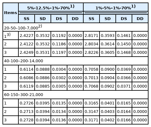
The accounting percentage derived from SS, SD, DS, and DD for the rate of inbreeding (ΔF) when the numbers of parents in SS, SD, DS, and DD are 40-100–200-14,000 is shown in Table 5. The accounting percentage in SS was the greatest of all the four selection paths for all two scenarios compared in the selection percentage in SS, SD, DS, and DD (that is, 5%-12.5%–1%-70% and 1%-5%–1%-70%), because the expectation of the square of lifetime long-term contribution of an individual was the greatest in SS of all the four selection paths (Table 4). The sum of accounting percentage in SS and SD was approximately 90% for ΔF, because the number of male parents in SS and SD was smaller than that of female parents in DS and DD and selection intensity in male parents is generally higher than that in female parents. In addition, the accounting percentage in each of the four selection paths when the numbers of parents in SS, SD, DS, and DD were 40-100–200-14,000 (Table 5) was approximately the same as the other scenario when the numbers of parents in SS, SD, DS, and DD were 20-50–100-7,000 or 60-150–300-21,000, although the accounting percentage in SS, SD, DS, and DD in the other scenarios was not shown. This is mainly because the expected contribution of an average parent (α) and the regression coefficient of the contribution of an individual on its selective advantage (β) are inversely proportional to the number of parents as explained previously in equation (1). Consequently, the accounting percentage derived from SS, SD, DS, and DD for the rate of inbreeding (ΔF), (that is, the relative magnitude of ΔF in SS, SD, DS, and DD), resulted in almost the same for all three scenarios compared in the numbers of parents in SS, SD, DS, and DD, even if the absolute magnitude of ΔF derived from each of the four selection paths differed in the number of parents in each of the four selection paths.

Table 5

The accounting percentage derived from SS, SD, DS, and DD for the rate of inbreeding (ΔF) when the numbers of parents in SS, SD, DS, and DD are 40-100–200-14,000

Correction derived from deviation from Poisson variance

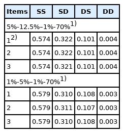
Corrections for deviations in the variance of the family size from independent Poisson variances (×10⁻⁴) approximated by binomial distribution are shown in Table 6. The magnitude approximated by binomial distribution under the assumed selection percentages in the SS, SD, DS, and DD selection paths of 5%-12.5%–1%-70% and 1%-5%–1%-70% varied from −0.29×10⁻⁴ to −0.88×10⁻⁴, and −0.04×10⁻⁴ to −0.12×10⁻⁴, respectively. In comparison, the rates of inbreeding with Poisson family size without correction shown in Table 2 varied from 0.2×10⁻² to 0.7×10⁻². Therefore, because the magnitude of correction was much smaller than that of the rates of inbreeding with Poisson family size without correction, correction is unnecessary; thus the rates of inbreeding without correction (Table 2) are reasonable rates of inbreeding. However, the method in terms of the factorial moments [10] should be examined to confirm that the magnitude of correction is much smaller than those of ΔF with Poisson family size without correction.

Table 6

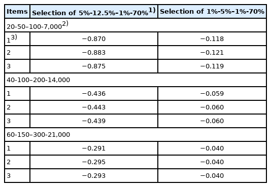
Correction factors for deviations of the variance of the family size from independent Poisson variances (×10⁻⁴) approximated by binomial distribution

Selection intensities and variance reduction coefficients should be adjusted by using the procedure from Wray and Thompson [4] in situations of few families with numerous candidates per family, for example, when the number of selected parents is only 5 or 10 [6]. Because we set the number of parents in SS at 20, 40, and 60, we did not adjust the selection intensity in the SS path. In addition, selection intensity in DD generally is much smaller than those in SS, SD, and DD selection paths. Consequently, when selection in DD is not performed, the selection intensity and reduction factor of the variance need to be set at zero in the DD selection path in the formula developed in the current study.