Multiple Linkage Disequilibrium Mapping Methods to Validate Additive Quantitative Trait Loci in Korean Native Cattle (Hanwoo)
Article information
Abstract
The efficiency of genome-wide association analysis (GWAS) depends on power of detection for quantitative trait loci (QTL) and precision for QTL mapping. In this study, three different strategies for GWAS were applied to detect QTL for carcass quality traits in the Korean cattle, Hanwoo; a linkage disequilibrium single locus regression method (LDRM), a combined linkage and linkage disequilibrium analysis (LDLA) and a BayesCπ approach. The phenotypes of 486 steers were collected for weaning weight (WWT), yearling weight (YWT), carcass weight (CWT), backfat thickness (BFT), longissimus dorsi muscle area, and marbling score (Marb). Also the genotype data for the steers and their sires were scored with the Illumina bovine 50K single nucleotide polymorphism (SNP) chips. For the two former GWAS methods, threshold values were set at false discovery rate <0.01 on a chromosome-wide level, while a cut-off threshold value was set in the latter model, such that the top five windows, each of which comprised 10 adjacent SNPs, were chosen with significant variation for the phenotype. Four major additive QTL from these three methods had high concordance found in 64.1 to 64.9Mb for Bos taurus autosome (BTA) 7 for WWT, 24.3 to 25.4Mb for BTA14 for CWT, 0.5 to 1.5Mb for BTA6 for BFT and 26.3 to 33.4Mb for BTA29 for BFT. Several candidate genes (i.e. glutamate receptor, ionotropic, ampa 1 [GRIA1], family with sequence similarity 110, member B [FAM110B], and thymocyte selection-associated high mobility group box [TOX]) may be identified close to these QTL. Our result suggests that the use of different linkage disequilibrium mapping approaches can provide more reliable chromosome regions to further pinpoint DNA makers or causative genes in these regions.
INTRODUCTION
In beef cattle, growth and carcass quality are very important traits, because of the relevance of these traits to economic profits for beef cattle farmers. Traditional breeding programs based on breeding values by best linear unbiased prediction (BLUP) using pedigree and phenotypic data has achieved significant genetic progress. For example, annual gains for carcass weight (CWT) and longissimus dorsi muscle area (LMA) in the 2000’s were 8 kg and 2.9 cm2, respectively, in Hanwoo (NIAS, 2009).
However, genomic prediction at a young stage can further accelerate genetic gain, because prediction errors at breeding age would be reduced by exploiting information on the value of every chromosomal fragment and on the transmission of chromosome fragments from parents to selection candidates (Garrick, 2011). Additionally, genome-wide prediction has the potential to reduce inbreeding rates because of the increased emphasis on own rather than family information (Daetwyler et al., 2011). Furthermore, quantitative trait loci (QTL) identification provides valuable information for understanding genetic mechanisms underlying beef phenotypes and for detecting causal polymorphisms, which subsequently can be utilized in beef industry through genome selection or gene-base selection (Misztal, 2011).
The availability of genome-wide single nucleotide polymorphism (SNP) panels enables detection of any SNP that is associated with a trait by a genome-wide association study (GWAS), which allows mapping QTL across the genome.
Several QTL mapping methods that exploited linkage disequilibrium between molecular markers and QTL have been suggested and applied (Zhao et al., 2007; Cierco-Ayrolles et al., 2010; Uleberg et al., 2010; Erbe et al., 2011; Sun et al., 2011). These methods are based on the assumption that saturated markers increase the feasibility of QTL detection using historical population-wide linkage disequilibrium, in which a marker allele is in linkage disequilibrium (LD) with the QTL allele across the entire population. The term, LD, implies disequilibrium of two loci due to physical linkage. However, disequilibrium can also exist between two loci that are physically unlinked, impairing reliability of LD-based QTL mapping, because the SNP far from the QTL may generate significant signals, i.e. false positive QTL.
To exclude false positive QTL, combined linkage and LD mapping methods were developed (Blott et al., 2003; Druet and George, 2010), in which linkage information, i.e. co-segregation of a marker and a QTL from parents to progeny, was exploited, so as to detect SNPs that are closely located (physically linked) to the QTL. Bayesian multiple regression methods consider prior information of QTL effect, which was based on previous results about genetic architecture of the traits of interest. Also, the Bayesian method allows a flexible criterion to control false positive QTL, i.e. probability of proportion of false positives among the significant QTL, while frequentist methods set stringent thresholds due to huge number of SNPs markers in the GWAS test (Fernando and Garrick, 2013).
The aim of this study was to detect additive QTL for growth and carcass quality traits in Korean cattle, Hanwoo, by applying three different genome wide association analyses, a linkage disequilibrium single locus regression method (LDRM), a combined linkage and linkage disequilibrium method (LDLA), and the Bayes Cπ method.
MATERIALS AND METHODS
Animals, phenotypes and molecular data
The steers (N = 486) for phenotype and molecular data were chosen among the progeny of candidate bulls for progeny testing in the Hanwoo Improvement Center of National Agriculture Cooperative Federation in Seosan, Chungnam province, Korea. The data set comprised 61 sires and their 486 steers that were born between spring of 2005 and fall of 2007. The number of steers for each of the 61 paternal sire families ranged from 2 to 13 with the average of eight steers. Some details about raising and management of the experimental population and data recording were described in Li et al. (2011).
Six traits for growth and meat quality were chosen: weaning weight (WWT), 365-d yearling weight (YWT), CWT after slaughter, backfat thickness (BFT), LMA, and marbling score (Marb). Details about summary statistics for the observed carcass quality traits were described in Li (2012).
A dense marker map covering the whole genome was embedded in the Illumina Bovine SNP 50K BeadChip (Matukumalli et al., 2009). Details of the SNP genotyping experiments were described in Lee et al. (2008). This quality control resulted in 39,501 useful SNPs which were used for further analysis. This subset of markers covers 2,543.6 Mb of the genome with 70.57±69.0 kb average adjacent marker spacing. For the SNPs analyzed in this study, the average observed heterozygosity was estimated at 0.37±0.12. The average minor allele frequency (MAF) of all SNPs before editing was 0.20 and using the filtered SNPs the averaged MAF increased to 0.27.
Models used
Three complementary approaches were used: i) linkage disequilibrium single locus analysis using the SNP_a option of Qxpak (5.03 version) software (Perez-Enciso and Misztal, 2011); ii) combined linkage disequilibrium and linkage analysis using linkage disequilibrium variance component mapping (LDVCM) software; iii) Bayesian analysis using the BayesCπ option of GenSel (http://bigs.ansci.iastate.edu/bigsgui/login.html). All analysis used appropriate fixed factors or covariates that were fitted in the models (p<0.05) using a general linear model procedure in SAS (SAS 9.1, SAS Institute Inc., Cary, NC, USA). Two fixed effects were fitted in the models: year and season of birth (5 levels) for all the traits and region where the steers were born (41 levels) for WWT, YWT, and Marb, and three covariates, weaning age for WWT, yearling age for YWT, slaughter age for CWT, BFT, and LMA, was also fitted. Pedigrees of the base population animals were traced back for 2 generations to create the numerator relationship matrix, and 1,033 animals were included in the pedigree analysis.
LDRM
First, linkage disequilibrium single locus regression (Grapes et al., 2004; Zhao et al., 2007) were performed.
Where y is the phenotypic record, μ is the average phenotypic performance, X is the design matrix of SNP genotype (e.g. individuals with marker genotypes ‘11’, ‘12’, and ‘22’ are assumed to have genetic values μkAA, 0, and μkBB), a is the fixed substitution effect for the SNP, Zu is the incidence matrix for animal effects, u is the infinitesimal genetic effect, which is distributed as
residual variance
LDLA
The LDVCM software has been essentially described (Kim and Georges, 2002; Blott et al., 2003). Briefly, the linkage phases of all sires and sons were determined by the approach of Druet and Georges (2010). Then, identity-by-descent (IBD) probabilities (ϕp) at the midpoint of each SNP interval (p) were computed for all pairs of haplotypes conditional on the identity-by-state status of flanking markers (Meuwissen and Goddard, 2001). A dendrogram was generated by using the unweighted pair group method with arithmetic mean (UPGMA) hierarchical clustering algorithm with 1-ϕp as the distance measure at QTL location (p). Starting at the ancestral node and sequentially descending into the dendrogram, all possible combinations of haplotype clusters were analyzed in place of individual haplotypes. This process identified the set of nodes at which the likelihood of the data were maximized.
To jointly exploit linkage disequilibrium (female meiosis) and linkage (male meiosis) information, the following mixed linear was used:
Where h is the vector of random QTL effects corresponding to the defined haplotype clusters. Zh is an incidence matrix relating maternal haplotypes of sons and sire haplotypes to individual sons. Likelihood ratio tests were performed by removing the haplotype cluster effects, and p-values were obtained assuming a x2 distribution of the likelihood ratio test with one degree of freedom. Association with FDR <0.01 on chromosome-wide level were considered significant.
BayesCπ
BayesCπ were developed from the BayesB and GBLUP approaches (Meuwissen et al., 2001) and was described in detail by Habier et al. (2011).
Where K is the number of SNPs, Xj is the vector of genotypes at SNPj, aj is the random substitution effect for the SNP, which condition on the variance
Information about particular genes, located near SNP significantly associated with each trait, was extracted from online sources (http://www.ensembl.org/index.html, http://www.genecards.org/cgi-bin/cardsearch.pl#top, and http://www.uniprot.org).
RESULTS AND DISCUSSION
The GWAS profiles of all additive SNP effects for each trait are divided into the different statistical models (Figure 1). All SNP effects in this report were additive as was expected because predicted transmitting ability predict only additive genetic merit.
Genome-wide scan for WWT, YWT, CWT, BFT, LMA, and Marb using the three approaches: LDRM, LDVCM, and BayesCπ. WWT, weaning weight; YWT, yearling weight; CWT, carcass weight; BFT, backfat thickness; LMA, longissimus dorsi muscle area; LDRM, linkage disequilibrium single locus regression method; LDVCM, linkage disequilibrium variance component mapping.
A total of 36 signal-trait combinations on 29 chromosomes crossed the chromosome-wide significance threshold by either LDRM or LDVCM, respectively (Tables 1 and 2). These signals in very close proximity to each other were often all significantly associated with a particular trait. This is because sets of SNPs that are physically located near the causal factor will tend to be in linkage disequilibrium. In this study, the same QTL was considered ‘detected’ if the significant signals were within a 1 Mb bracket. Therefore, the total number of distinct identified QTLs is 17. Of these 17 QTLs, 5 were commonly detected by both methods, while 7 and 5 were solely detected by LDRM and LDVCM, respectively.
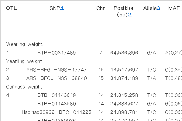
The additive QTL and SNP position that were detected for growth and carcass quality traits using LDRM analysis
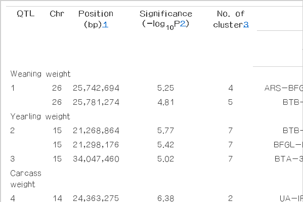
The additive QTL and SNP position that were detected for growth and carcass quality traits using LDVCM analysis
Subsequent BayesCπ provides a reference for validation of association results, using a cut-off of the top 5 variances of 10-SNP windows (Table 3). The associated signal plots show in Figure 2, which provide a visualization of whether the consistency QTL were detected by three approaches. The consistency of QTL results obtained from the same dataset using different statistical approaches can provide more reliable chromosome regions to further pinpoint DNA makers or causative genes in these regions.

The additive QTL and SNP position that were detected for growth and carcass quality traits using BayesCπ analysis
QTL profile (upper) and annotation (lower) of the detected SNPs associated with BFT on BTA6, WWT on BTA7, CWT on BTA14 and BFT on BTA29. QTL, quantitative trait loci; SNPs, single nucleotide polymorphisms; BFT, backfat thickness; BTA, Bos taurus autosome; WWT, weaning weight; CWT, carcass weight.
Quantitative trait loci analysis by LDRM and LDLA
The single marker regression based on LD is shown in Table 1. The LDRM found 17 significant SNP associations, including 1 for WWT, 2 for YWT, 5 for CWT, 8 for BFT, and 1 for LMA. Ten of these SNPs were in agreement with QTL previously reported in the literature, including 1 for WWT, 1 for YWT, 5 for CWT, and 3 for BFT (Mizoshita et al., 2005; McClure et al., 2010). Further, 3 of the 17 detected SNPs are located within the regions of known genes, and the others are 12,174 to 459,952 bp away from the nearest known genes. Among these 17 SNPs, there are 5, 2 SNPs located within a 2 Mb (between 24.31 to 25.29Mb) for CWT on Bos taurus autosome (BTA) 14, and a 0.2Mb (between 52.72 and 52.88Mb) for BFT on BTA13, and this indicated that they are associated with the same QTL.
LDLA results for growth and carcass quality using LDVCM are in Table 2. The LDVCM detected a total of 19 significant signals, including 2 for WWT, 3 for YWT, 2 for CWT, 11 for CWT, and 1 for Marb. Ten of these signals were in agreement with QTL previously reported in the literature, including 2 for WWT, 2 for YWT, 2 for CWT, and 3 for BFT (Mizoshita et al., 2005; McClure et al., 2010). Further, 5 of the 19 detected SNPs are located within the regions of known genes, and the others are 526 to 494,805 bp away from the nearest known genes. In particular, many significant signals (15 out of 19) were located in close distances: i.e. 5 SNPs are located within 0.2 Mb (between 26.24 to 26.45 Mb) for BFT on BTA29, which harbors the neuron navigator 2 (NAV2) gene.
Quantitative trait loci analysis by BayesCπ
BayesCπ analysis fitted all the SNPs simultaneously. Examination of genetic variance associated with 10-SNPs windows across the genome were chosen by the top 5 (Table 3, Figure 1). The largest differences were an increase in genetic variance associations found per traits: the 64.1 to 64.9 Mb region of BTA1 for WWT, 60.7 to 61.6 Mb region of BTA4 for YWT, 159.4 to 160.2 Mb region of BTA1 for CWT, 0.5 to 1.5 Mb region of BTA6 for BFT, 28.1 to 29.2 Mb region of BTA17 for LMA, and 159.4 to 160.2 Mb of BTA1 for Marb. Some SNPs windows affected more than one carcass quality trait, including 24.7 to 25.4 Mb for BTA 14 (CWT and LMA), 35.6 to 36.5 Mb for BTA14 (CWT and Marb), 25.2 to 25.9 Mb for BTA27 (CWT and Marb) and 159.4 to 160.2 Mb for BTA1 (CWT, LMA, and Marb) (Stone et al., 1999; Li et al., 2004; Mizoshita et al., 2004; Mizoshita et al., 2005; Morris et al., 2009; McClure et al., 2010).
Comparison of result
The 17 QTL detected by LDRM or LDVCM were integrated using the BayesCπ analysis to remove possible redundancies among those QTL. The purpose of QTL mapping is as a first step towards the identification of QTL locations for further investigation by molecular geneticists. Therefore, agreement of the location of positive signals between the three detection methods was evaluated. The visual agreement of the information generated by these methods is evident from Figure 2. Four QTL from these three methods had the high concordance locations and statistics found in 64.1 to 64.9 Mb for BTA7 for WWT, 24.3 to 25.4 Mb for BTA14 for CWT, 0.5 to 1.5 Mb for BTA6 for BFT and 26.3 to 33.4 Mb for BTA29 for BFT. As shown in Figure 2 and Table 1, 2, and 3, the QTL for WWT was positioned within 64.1 to 64.9 Mb, one of the gene glutamate receptor, ionotropic, ampa 1 (GRIA1), that encodes glutamate receptor 1. The QTL for CWT was detected in the proximal region (24.3 to 25.4 Mb) of BTA14, which encompasses family with sequence similarity 110, member B (FAM110B), ubx domain protein 2B (UBXN2B), and thymocyte selection-associated high mobility group box (TOX) as positional and functional candidate genes for the CWT QTL in cattle. A QTL for BFT was detected in the proximal region (0.5 to 1.5 Mb) of the BTA 6, in which Locus (LOC) 100139637 gene was located. Another QTL was detected for Marb in the proximal region of the BTA29 (26.3 to 33.4 Mb), around which NAV2 gene was located. These QTL locations that were found by each method were as expected because the chromosomes were suspected to contain QTL.
Previous work has shown that these three methods belong to three distinct analytical methods, i.e. LDRM tests a single marker at a time and regards the markers as independent of all other markers (Grapes et al., 2004; Zhao et al., 2007; MacLeod et al., 2010), LDVCM tests the midpoint of the marker brackets, which corresponded best when the QTL was masked between analyzed markers(Kim and Georges, 2002; Blott et al., 2003), and BayesCπ test the effects of all markers, which are fitted simultaneously. However, QTL with large effects can be detected by both the Bayesian shrinkage and linear regression mapping methods. By specifying proper prior distributions for SNP effects, the ignorable small SNP effects are coerced to zero and only SNPs with larger effects on the phenotype are fitted in the model, hence Bayesian shrinkage analysis could reduce possible spurious QTL effects by adjusting all other QTL effects. This was also explained by Xu (2003) and Sun (2011). Therefore, here we attempted to minimize the number of false positives by combined these three methods result.
The establishment of a threshold is a complicated issue and has a profound influence on the results, especially when methods with different nature of scores are compared. False discovery rate derived threshold takes into account the number of tests that are performed as well as how significant one test is relative to the others in multiple comparison procedures. Two levels of significant controls were used in LDRM and LDVCM analysis based on genome-wide (FDR<0.05) and chromosome-wide (FDR<0.01) type I errors, which were computed for all SNP (Fernando et al., 2004). Usually, significance tests are not required in Bayesian analysis; only frequentists emphasize significance tests. However, to facilitate comparison with other methods, we accumulated the effects of adjacent SNPs together into a genomic window and then chose the top 5 as cut-off the criterion to detect QTL in BayesCπ. Figure 2 clearly shows the major peaks in BayesCπ coincide with LDRM and LDVCM. Therefore, these present findings together with those of Sun et al. (2011) suggest that the genetic variances estimated by BayesCπ including all markers without polygenic effects can exploit the generated gene discovery knowledge.
Table 1 and 3 show that the SNP effects explained by BayesCπ were smaller than those by LDRM. These result were not surprising because we performed LDRM in the way of SNP by SNP individually via regressing the traits on the genotypes of a SNP and thus ignored all possible SNP-covariate or SNP-SNP pairs for interaction effect, leading to the model effect acting as the effect of the marker, particularly with small mapping population (Xu, 2003; Hoggart et al., 2008). Additionally, the SNP effect can be overestimated in LDRM, especially when the effect of a SNP is small, this is due to the so called Beavis effect (Xu, 2003). Therefore, the work in this study is more related to QTL position rather than the precise estimation of their effects.
Our study successfully uncovered many variants related to QTLs. However, the traits YWT, CWT, and BFT measured in Hanwoo have QTL with larger additive effects than WWT, LMA, and Marb. Several explanations have been proposed for our scant outcomes from genetic markers. First, the currently identified SNPs might not fully describe genetic diversity. For instance, these SNPs may not capture some forms of genetic variability that are due to copy number variation. Second, genetic mechanisms might involve complex interactions among genes and between genes and environmental conditions, or epigenetic mechanisms which are not fully captured by additive models. However, opportunities may exist for improving predictions by exploiting additive genetic variation. A third explanation—the one we focus on here lies—in the limitations posed by the genetic models and statistical methods.
CONCLUSION
No linkage disequilibrium mapping method tested in this study outperformed the others, but it is interesting that the positions of the SNP selected by the different models (LDRM, LDLA, BayesCπ) were close. Some well-known candidate genes for the traits of interest were located close to these QTL. Four major additive QTL in each analysis had high concordance including 64.1 to 64.9 Mb for BTA7 for WWT, 24.3 to 25.4 Mb for BTA14 for CWT, 0.5 to 1.5 Mb for BTA6 for BFT and 26.3 to 33.4 Mb for BTA29 for BFT. We suggest the use of combined different LD mapping approaches can provide more reliable chromosome regions to further pinpoint DNA makers or causative genes in these regions.
ACKNOWLEDGMENTS
This work was supported by Shanxi Scholarship Council of China 2013-072 (YL) and by the Natural Science Foundation of Shanxi 2014011030-4 (YL). Dr. Jong-Joo Kim is supported by the Technology Development Program for Agricultural and Forestry, Ministry of Agriculture, Forestry and Fisheries, Republic of Korea, 2014.
Notes
CONFLICT OF INTEREST
We certify that there is no conflict of interest with any financial organization regarding the material discussed in the manuscript.